A weak Alpha signal invites familiar explanations: too little analyte, a damaged reagent, perhaps a sample that never contained much of the thing being measured. If the signal rises when the sample is diluted, low analyte concentration becomes a less convincing explanation.
In a sandwich Alpha assay, a concentrated sample can produce less light than a dilute one. Excess analyte occupies the binding partners separately, reducing the productive bridges between donor and acceptor beads. The high-dose hook effect gives a single low signal two possible concentration ranges. One is below the useful range. The other can be far above it. [1]
That ambiguity is easy to overlook on a plate full of plausible numbers. A low result still looks like a result. Nothing in the exported count value says which side of the curve supplied it.
Too many molecules for a productive encounter
Consider a sandwich format in which one recognition reagent connects analyte to a donor bead and another connects it to an acceptor bead. A productive complex brings the beads close enough for donor-generated singlet oxygen to initiate the acceptor signal. As analyte rises through the useful range, more productive complexes form.
At sufficiently high analyte concentration, many capture sites acquire separate analyte molecules. Occupancy can remain high while productive bead bridging falls. More analyte can therefore mean fewer light-producing complexes. The AlphaScreen practical guide describes this behavior and recommends titration when establishing useful component concentrations. [1]
The details depend on reagent affinity, valency, concentrations and the order of additions. A competitive assay intentionally designed to lose signal as analyte rises has a different interpretation. The word “hook” should be reserved for evidence of the relevant excess-component behavior, rather than applied to every downward curve.
One signal, two concentrations
An illustrative curve makes the ambiguity visible. Let x be analyte concentration divided by an arbitrary peak concentration of 10 nM. Define a normalized signal:
This is a schematic, not a fitted Alpha mechanism or a kit calibration. It rises to one at x = 1 and then falls. Concentrations equally far above and below the peak on a logarithmic scale give identical signals. Thus 1 nM and 100 nM both produce approximately 0.331 in this constructed example.
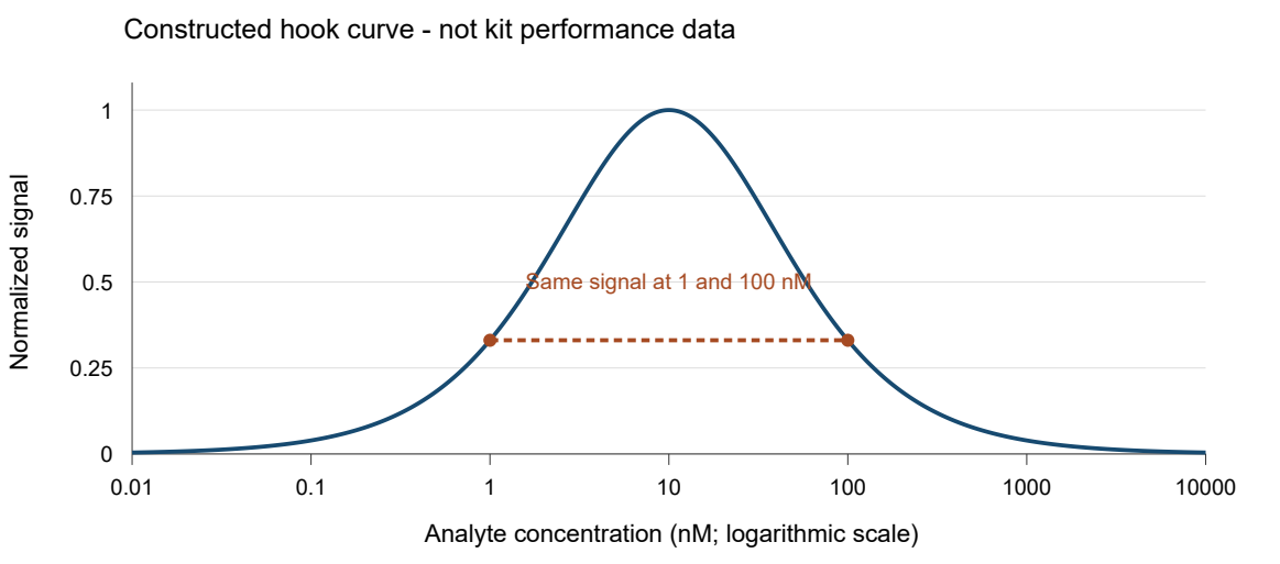
Start with a hypothetical 1,000 nM sample and prepare the following dilutions before adding the detection reagents. Keep final reagent concentrations, volumes and incubation conditions constant.
| Sample dilution | Analyte in the model | Normalized signal |
|---|---|---|
| Undiluted | 1,000 nM | 0.039 |
| 1:10 | 100 nM | 0.331 |
| 1:100 | 10 nM | 1.000 |
| 1:1,000 | 1 nM | 0.331 |
| 1:10,000 | 0.1 nM | 0.039 |
The first two dilution steps make the sample brighter. Further dilution brings it down the rising-concentration branch toward the blank. Its initial weak signal was compatible with a very large amount of analyte.
The equal signals in the table can also lead to a large reporting error. If the 1:10 dilution, containing 100 nM, is interpreted using the low-concentration branch, the calibration assigns 1 nM. Multiplying by ten reports 10 nM in the original sample, a hundredfold underestimate. Applying the dilution factor correctly cannot repair selection of the wrong branch.
A tidy standard curve leaves a question open
The AlphaLISA human IL6 AL223 manual instructs users to exclude standard concentrations beyond the hook point when fitting its specified calibration model. That gives a usable monotonic calibration. It leaves the analyst responsible for establishing that unknown samples belong on the fitted branch. The manual also calls for a standard curve for each experiment and standards in a matrix similar to the samples. [2]
The fitted standard curve alone cannot establish which branch an unknown sample occupies. Keep the wider development titration as evidence of where the response turns. For samples that may exceed the validated range, test multiple dilutions and seek agreement in the dilution-corrected concentration within a predefined acceptance tolerance.
Avoid quantifying close to a flat peak, where a small signal error can correspond to a large concentration error. Agreement among several useful dilutions is more convincing than one number that happens to fall between the calibration limits. The useful range must support precision and recovery; merely detecting a signal above blank does not establish reliable quantitation.
A second bookkeeping problem lurks in the phrase “final concentration.” Many kit curves label the concentration of the sample aliquot before detection reagents are added. If standards and samples both undergo that reagent addition, its dilution is already represented in the calibration. Follow the kit's concentration convention and correct additional sample predilution once. Applying that same dilution a second time overstates the sample concentration.
Dilution changes more than analyte
A real sample carries salt, protein, detergent and sometimes colored or reactive material. Dilution lowers those components alongside the analyte. Relief of quenching, singlet-oxygen interference or another matrix effect can also increase the signal. A rising response after dilution is a reason to investigate, rather than a diagnosis by itself.
Begin with the actual dilution buffer and the matrix the kit supports. Compare dilution behavior with analyte standards prepared in a suitably matched matrix. Where feasible, maintain the relevant background using analyte-depleted matrix, verifying that depletion has not introduced a new difference. Match sample volume and final bead concentrations across the comparison.
Spike recovery adds useful evidence, especially across several dilution levels, but it has limits. A purified spike can behave differently from endogenous analyte associated with other proteins. A spike can also push a sample further into antigen excess. Interpret the result with the broader concentration series and, when needed, a detection-interference control appropriate to the assay architecture.
The practical troubleshooting sequence is to establish a broad response curve, examine sample dilution, and then vary matrix and detection conditions separately. Record what changes in each comparison. Diluting an already assembled bead mixture changes bead concentration and binding equilibria; it is a different experiment from prediluting the sample before the standard protocol.
Keep detector compression separate
Detector nonlinearity can distort a concentration series, particularly near the bright end. A wide, verified linear measurement range reduces that complication. There is, however, an important constraint on the explanation: ordinary monotonic compression cannot, by itself, make less incident light produce a larger raw output. It squeezes differences while preserving their order.
If dilution produces higher raw counts, something more must have changed: the chemistry, matrix, acquisition settings or a nonmonotonic overload behavior. By contrast, an increase in the dilution-corrected estimate can occur when dilution relieves ordinary compression. Keep raw signal and corrected concentration in separate columns before deciding which observation needs explaining.
Check the reader's response using a qualified reference or attenuation procedure suitable for that detection mode, within specified operating conditions. A biochemical analyte dilution simultaneously changes the light-producing reaction and therefore cannot independently prove detector linearity. Nor does the absence of a saturation warning establish proportional response.
Bright neighboring wells introduce another complication. Optical leakage can lift a weak sample above its own signal. Preventing those photons from entering the measurement is preferable to relying entirely on subtraction: an average correction can remove an estimated contribution while leaving photon noise and uncertainty in that estimate. Include representative bright-neighbor arrangements when qualifying low samples on a screening plate.
Give the dilution series the same thermal history
The AL223 manual warns that signal varies with temperature and incubation time and calls for consistent conditions across plates. Its illustrated procedure uses incubations at 23°C. [2] A dilution series read while successive plates warm in the chamber combines a concentration experiment with a temperature experiment.
Equilibrate samples and detection reagents as the kit requires, maintain the specified timing, and read near the validated room-temperature condition in a stable chamber. For a long batch, inspect distributed controls and record plate order. Equal incubation labels do not guarantee equal liquid temperatures after different waits in a stack.
For an unfamiliar sample, retain the dilution series alongside the reported concentration. The pattern contains information that the final number discards. A specimen that gets brighter on dilution deserves enough additional points to show where the signal turns and where corrected concentrations begin to agree.
References
1. PerkinElmer. AlphaScreen practical guide. Hook effect: PDF p. 21 / printed p. 15. Temperature and assay interference: PDF pp. 30–32.
2. Revvity. AlphaLISA human IL6 kit AL223 manual. Manual-AL223-VRB1. Matrix and timing guidance: pp. 5–7; post-hook standard exclusion, dilution correction and concentration reporting: p. 8. Assay-specific instructions; the constructed curve in this essay is not IL6 performance data.